Tutorial 3 — Foot-traffic flow analysis in Cambridge

This tutorial examines the una.RunFlow() engine for modeling active-mobility trips over networks, using walking trips in Cambridge, MA. Steps (a)–(i) use a single origin (MIT_SAP) and two named destinations; step (j) scales to every Cambridge building centroid; step (k) automates multiple flows from a pairings CSV.

Data files (in docs/Boston/ (in the UNA repository)):

Network (a–h): 20260703_PercLenNetwork_InnerCore.geojson — 69,957 pedestrian-network edges (2D; a 3D twin is used in step g).
Origin (a–h): MIT_SAP_flow_origin.geojson — MIT School of Architecture + Planning, a single point with weight = 100.
Destinations (a–h): HarvardHC_and_GSD.geojson — two points: Harvard_HousingCtr (2,195.1 m from MIT_SAP along the network, weight 1) and Harvard_GSD (2,585.6 m, weight 3).
Step (i): Cambridge_building_centroids.geojson (14,751 buildings) → Cambridge_metro_stations.geojson (18 rapid-transit stations, weighted by weekly_departures).

Note

Two flow engines. Since v2.5.5, UNA ships two flow engines selected by /user_guide/settings_reference:flow_engine. The default is "aggregate_flow" — a scalable engine that spreads each trip across the full detour envelope without enumerating discrete paths (see Aggregate flow (gradient-overlap method)). Steps (a)–(h) teach the K-alternative-routes engine, so the script sets flow_engine = "k_alternatives" explicitly; step (i) switches to the aggregate engine on identical inputs, and steps (j)–(k) continue with it. All concepts introduced here — decay, weights, Huff destination choice, detour envelope — apply to both engines.

(a) Shortest path only — one simple trip 

Emit ONE trip from MIT_SAP to its closest reachable destination along the shortest path. A useful sanity check before adding realism.

from urban_network_analysis import UNA
una = UNA()

una.settings.data_folder       = r"Boston"
una.settings.network_file      = "20260703_PercLenNetwork_InnerCore.geojson"
una.settings.origins_file      = "MIT_SAP_flow_origin.geojson"
una.settings.destinations_file = "HarvardHC_and_GSD.geojson"
una.settings.search_radius     = 4000
una.settings.flow_engine       = "k_alternatives"  # explicit — v2.5.5 defaults to "aggregate_flow"

una.settings.flow_detour_ratio         = 1.0    # shortest path only
una.settings.use_nearest_destination   = True   # nearest destination only
una.settings.flow_decay                = False
una.settings.flow_origin_weights       = False
una.settings.flow_destination_weights  = False
una.settings.turns                     = False
una.settings.elevation                 = False

una.RunFlow()

Metric	Value
Max flow (edge)	1.0000
Edges with flow > 0	49 (of 69,957)

49 edges form the shortest path to Harvard_HousingCtr (the closer destination); each carries exactly one trip’s worth of flow. Harvard_GSD is ignored because use_nearest_destination=True restricts the analysis to the single closest destination.

(b) Add distance decay, β = 0.001 

The trip volume is reduced by exp(−β·d) = exp(−0.001 × 2,168) ≈ 0.114.

una.settings.flow_decay       = True
una.settings.flow_decay_curve = "exponential"
una.settings.gravity_beta     = 0.001

Metric	Value
Max flow (edge)	0.114
Edges with flow > 0	49

Same 49-edge path; every edge now carries ~11 % of a trip.

(c) Add origin weight — 100 residents at MIT_SAP 

una.settings.flow_origin_weights  = True
una.settings.origin_weight_column = "weight"

Metric	Value
Max flow (edge)	11.42
Edges with flow > 0	49

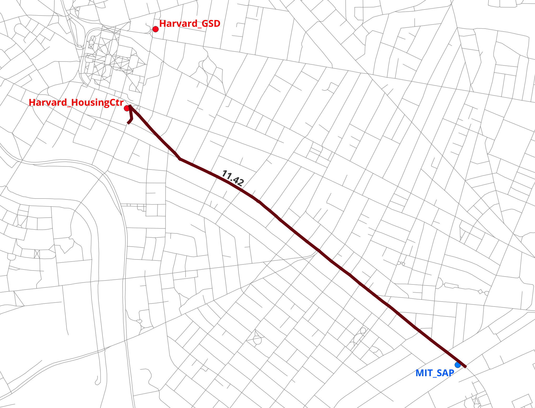
Max flow jumps to 100 × 0.114 = 11.42 — origin weights are a pure multiplier on trips generated.

(d) Loosen the envelope — detour_ratio = 1.2 

Allow alternatives up to 20 % longer than shortest. Trip volume stays constant but splits across K alternative routes.

una.settings.flow_detour_ratio = 1.2

Metric	Value
Max flow (edge)	11.42 (trunk edges)
Edges with flow > 0	114

2.3× as many edges carry flow, concentrated along the Massachusetts Avenue corridor shared by multiple alternatives.

(e) Include both destinations 

una.settings.use_nearest_destination = False

Metric	Value
Max flow (edge)	11.42
Edges with flow > 0	214

Harvard_GSD now receives flow too. Both destinations carry unit weight, so Harvard_HousingCtr’s shorter distance (decay 0.111 vs 0.075) gives it the larger share.

(f) Huff destination choice — destination weights on 

Harvard_GSD is 3× more attractive (weight 3 vs 1). Allocation follows gravity[d] = weight[d] × exp(−β·d), normalized across destinations.

una.settings.flow_destination_weights  = True
una.settings.destination_weight_column = "weight"

Destination	gravity	trip share
Harvard_HousingCtr	1 × 0.111 = 0.111	≈ 33 %
Harvard_GSD	3 × 0.075 = 0.226	≈ 67 %

Max edge flow stays constant at 11.42, but more flow now ends up at the GSD and less at the Housing Center. This is Huff destination choice in action: the 3× weight overcomes the 18 % distance penalty.

(g) Enable elevation, penalty = 4 

una.settings.network_file = "20260703_PercLenNetwork_InnerCore_3D.geojson"
una.settings.elevation         = True
una.settings.elevation_penalty = 4

Metric	Value
Max flow (edge)	9.93
Edges with flow > 0	212

Max flow falls from 11.42 to 9.93 (~13 %): uphill segments on the routes toward Harvard raise the perceived distance to both destinations, so the distance-decay factor drops and fewer trips are generated. The set of routes barely changes (214 → 212 edges) — Cambridge is comparatively flat along this corridor — but every route carries proportionally less volume. Subtler than Beacon Hill would be, but measurable.

(h) Enable turns, threshold = 45°, penalty = 35 

una.settings.turns          = True
una.settings.turn_threshold = 45
una.settings.turn_penalty   = 35

Metric	Value
Max flow (edge)	9.93
Edges with flow > 0	179

Nonzero edges drop from 212 to 179 — turn penalties eliminate the twisty alternatives, leaving the straight-through routes along Massachusetts Avenue. Flow concentrates on fewer edges: the corridors pedestrians actually walk when minimizing turns are much narrower than raw topology suggests.

(i) Switching to the aggregate-flow engine 

Everything so far enumerated K discrete alternative routes per OD pair. UNA’s second engine — aggregate_flow, the default since v2.5.5 — models the same trips without enumerating paths: each trip’s volume is spread continuously over every network segment that can lie on a route within the detour envelope, weighted by how much of a detour passing through that segment implies (see Aggregate flow (gradient-overlap method)). Keeping every input from (h) identical, the switch is one line:

una.settings.flow_engine = "aggregate_flow"

una.RunFlow()

Metric	k_alternatives (h)	aggregate_flow (i)
Max flow (edge)	9.93	9.93
Edges with flow > 0	179	986

The maximum is identical — both engines conserve trip volume, so the trunk segments near the origin and destinations carry the same full load. The difference is coverage: instead of loading K discrete routes, the aggregate engine loads the entire feasible envelope — 986 edges versus 179 — with volume tapering smoothly from the shortest path outward.

../_images/t3_image7.png — Aggregate flow from MIT_SAP to the two Harvard destinations with inputs identical to (h). The shortest-path trunk carries nearly the full 9.93 trip volume end to end, while flow tapers off across the surrounding detour envelope — hundreds of segments carry small fractions of a trip instead of K discrete routes carrying all of it.

How sharply the flow tapers is governed by /user_guide/settings_reference:flow_path_detour_penalty (default "logistic", midpoint /user_guide/settings_reference:flow_route_enumeration_logistic_midpoint); a stronger penalty concentrates flow near the shortest route, a weaker one spreads it evenly across the envelope.

Two practical notes. The aggregate engine scales far better with origin count — it needs no per-path enumeration — which is why the remaining steps use it. And it produces no discrete routes, so the route-geometries export of /user_guide/settings_reference:flow_output_routes requires k_alternatives.

(j) Many-to-many — 14,751 buildings → 18 metro stations 

Scale to every Cambridge building reaching every rapid-transit station within a 600 m walk — the configuration an agency would use to map “which streets carry the most foot traffic from homes to transit?” (turns and elevation off for fast iteration; the engine stays aggregate_flow from step (i) — exactly the workload it is built for):

una.settings.origins_file             = "Cambridge_building_centroids.geojson"
una.settings.origin_weight_column     = "Count"
una.settings.destinations_file        = "Cambridge_metro_stations.geojson"
una.settings.destination_weight_column = "weekly_departures"
una.settings.search_radius            = 600
una.settings.turns     = False
una.settings.elevation = False

Metric	1k-building sample	Full 14,751 (estimate)
Run time	~2 s	well under a minute on a laptop
Edges with flow > 0	937	≈ 6,000–8,000 (~9–11 %)
Max edge flow	51.26	~750

../_images/t3_image8.png — Building-to-transit flows across Cambridge. Each station collects walking trips from the buildings within its 600 m envelope, forming a distinct catchment; flow intensifies along the approach corridors toward each station entrance — Porter, Harvard, and Central show the strongest trunk loads.

The classic long-tailed distribution of pedestrian flow: trunk corridors — Massachusetts Avenue, Broadway, Cambridge Street — dominate, surrounded by a much larger network of low-flow neighborhood streets. (With k_alternatives the same sample takes ~6× longer and loads fewer edges — the aggregate engine’s envelope coverage and speed are exactly why it is the default at this scale.)

(k) Automating multiple flows with UNA_Batch.py 

A planning study typically wants the same analysis run on several origin/destination pairs. UNA_Batch.py lists every flow as a row in a pairings CSV; internally it calls una.RunBatch("flow", pairing_file=...), which runs each row and — because rows set batch_composite_output = TRUE — merges every flow’s per-edge result into a composite output.

The Boston pairings CSV (Boston/Boston_Flow_pairings.csv) has two flows:

name	origins (weight)	destinations (weight)	radius
homes_to_transit	Cambridge_building_centroids_pop2020 (pop2020)	Cambridge_transit_stations (weekly_departures)	600 m
schools_to_transit	schools_cambridge (weight)	Cambridge_transit_stations (weekly_departures)	400 m

Note the destination layer: unlike step (j), which used only the 18 rapid-transit (metro) stations, both rows here target Cambridge_transit_stations.geojson — 434 stops including bus stops as well as metro stations, each weighted by its weekly_departures. That is why the resulting flow map covers nearly the whole city rather than a handful of station catchments.

Shared columns across rows include flow_decay = TRUE, flow_decay_curve = exponential, gravity_beta = 0.001, flow_detour_ratio = 1.2, batch_composite_output = TRUE, and batch_composite_result_column = edge_flow. Rows without a flow_engine column run the default aggregate_flow engine; the flow_n_alternatives and flow_alternative_penalty_factor columns in the CSV apply only when a row sets flow_engine = k_alternatives.

The full UNA_Batch.py script — edit the three path constants and the analysis type at the top, everything else stays as shipped:

from urban_network_analysis import UNA

# --------------------------------------------------------------
# EDIT THESE THREE VALUES
# --------------------------------------------------------------

DATA_FOLDER   = r"Boston"
PAIRINGS_FILE = r"Boston/Boston_Flow_pairings.csv"
OUTPUT_FOLDER = r"Boston/Results"

# Which analysis to run per row — must match the metric in your
# pairings CSV:
#   "accessibility"  — for reach / gravity_* / knn_access composites
#   "flow"           — for edge_flow or node_flow composites
ANALYSIS = "flow"

# --------------------------------------------------------------
# Run the batch (per-row files + composite edge-flow file)
# --------------------------------------------------------------

una = UNA()
una.settings.data_folder   = DATA_FOLDER
una.settings.output_folder = OUTPUT_FOLDER

una.RunBatch(ANALYSIS, pairing_file=PAIRINGS_FILE)

All the per-flow settings — origin/destination files and weights, search_radius, decay parameters, flow_detour_ratio, batch_composite_output — come from the pairings CSV rows, not from the script. Run it with:

python UNA_Batch.py

Per-row outputs land in Results/<name>_<timestamp>/; the composite file has one edge-flow column per row plus a final composite_sum column — ideal for QGIS overlays that toggle between flow types or compare their sum/difference per edge. (node_flow also works as the composited metric for intersection-level composites.) See Project workflow — RunBatch().

../_images/t3_image9.png — The batch’s `composite_sum` rendered in QGIS: homes-to-transit and schools-to-transit flows summed per edge across all of Cambridge. Because the destination set now includes all 434 bus and metro stops, flow covers nearly the whole street network instead of a handful of station catchments — while still concentrating along Massachusetts Avenue through Porter, Harvard, and Central, and on the approach streets to Kendall/MIT and Lechmere.

What we covered 

From one trip on one shortest path to a city-scale model: shortest path (a), distance decay (b), origin weights (c), alternative paths (d), multiple destinations (e), Huff destination choice (f), elevation (g), turns (h), the aggregate-flow engine (i), many-to-many (j), and CSV-driven batching (k). The same parameters mean the same things at every scale — only run time and output size change.

Next: Tutorial 4 — Evaluating a design intervention — using flow to evaluate a concrete urban-design intervention. For the scalable engine behind the new default, see Aggregate flow (gradient-overlap method).