Tutorial 2 — Accessibility step-by-step (Boston)
This tutorial builds an accessibility analysis on the Boston inner-core
data in nine progressive steps. Each step changes one or two settings
and shows what happens to the result. Open UNA_Workspace.py in VS
Code with the una conda environment active; modify the script in
place and rerun python UNA_Workspace.py after each variation.
The data files live in docs/Boston/ (in the UNA repository):
Network (steps a–f, h):
20260703_PercLenNetwork_InnerCore.geojson— 69,957 pedestrian-network edges covering the Boston inner core (Cambridge + Boston core), 2D.Network (step g, elevation):
20260703_PercLenNetwork_InnerCore_3D.geojson— the same network with elevation sampled at every vertex (x, y, z).Origins (steps a–e):
MIT_SAP_Harvard_GSD.geojson— two points: the MIT School of Architecture + Planning and the Harvard Graduate School of Design.Destinations:
MA_transit_stations.geojson— 6,919 transit stops across the MBTA region, with aweekly_departuresattribute.Origins (steps f–h):
Cambridge_building_centroids.geojson— 14,751 building centroids across Cambridge.
Each step below shows only the settings that change relative to the previous step.
(a) Reach to transit stops — two origins, radius 400 m
The simplest possible accessibility analysis: count transit stops reachable within a 400 m network walk, with no destination weighting.
from urban_network_analysis import UNA
una = UNA()

una.settings.data_folder       = r"Boston"
una.settings.network_file      = "20260703_PercLenNetwork_InnerCore.geojson"
una.settings.origins_file      = "MIT_SAP_Harvard_GSD.geojson"
una.settings.destinations_file = "MA_transit_stations.geojson"
una.settings.search_radius     = 400

una.settings.calculate_reach               = True
una.settings.calculate_exponential_gravity = False
una.settings.calculate_logistic_gravity    = False
una.settings.calculate_knn_access          = False

una.settings.origin_weight_column      = "Count"
una.settings.destination_weight_column = "Count"

una.RunAccessibility()
Origin |
Reach |
|---|---|
MIT_SAP |
7.00 |
Harvard_GSD |
9.00 |
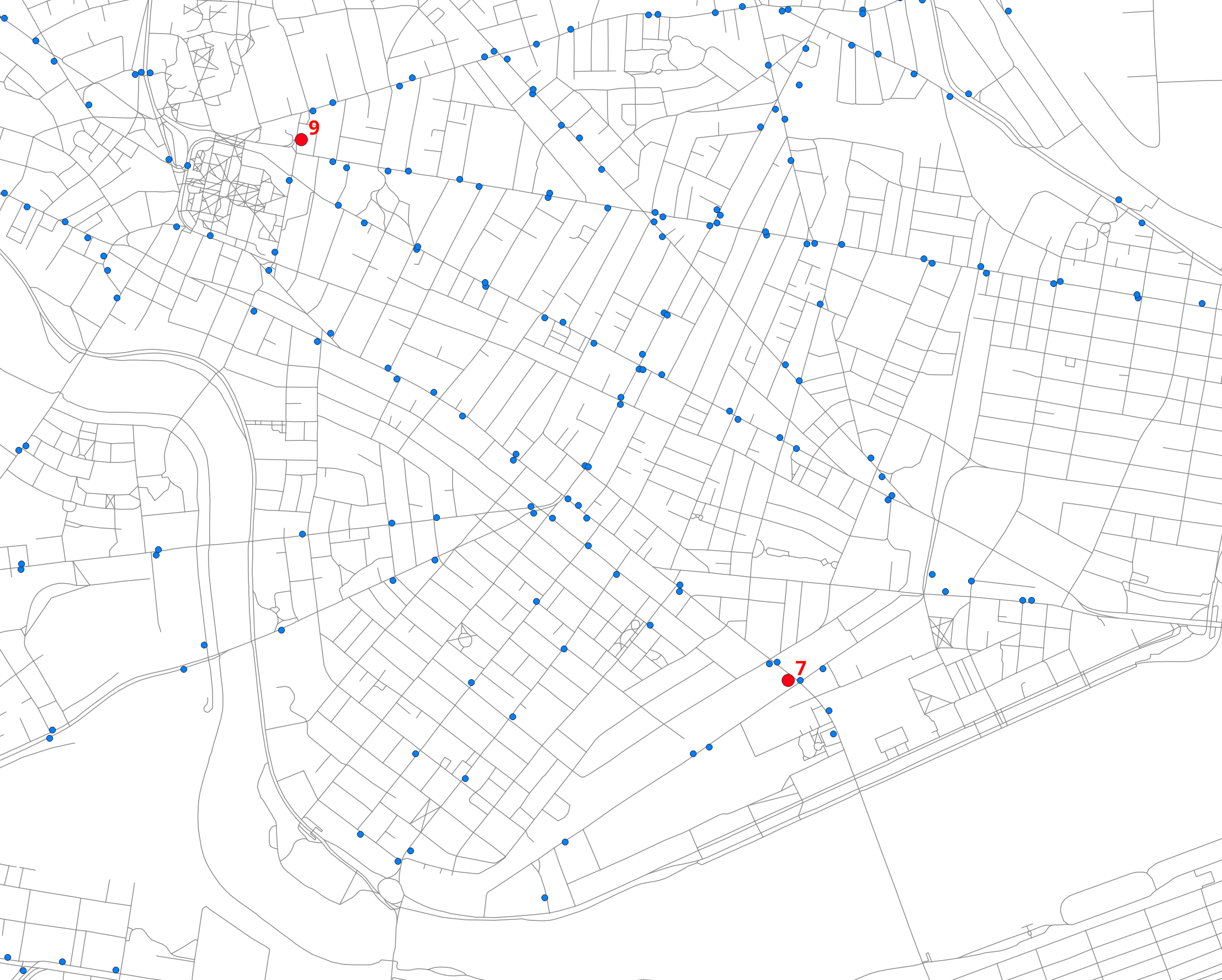
Within a 400 m walk, MIT_SAP reaches 7 transit stops and Harvard_GSD reaches 9 — raw counts, every stop contributing 1.
(b) Add destination weights (weekly_departures)
Weight each stop by its weekly departures — a proxy for service frequency. Reach becomes a weighted sum rather than a raw count.
una.settings.destination_weight_column = "weekly_departures"
Origin |
Reach |
|---|---|
MIT_SAP |
3,456.00 |
Harvard_GSD |
3,427.00 |

MIT_SAP’s fewer stops turn out to carry almost the same aggregate service level as Harvard’s more numerous ones.
(c) Add Gravity (exponential), β = 0.001
Gravity additionally penalizes distance — each destination contributes
weight × exp(−β·d). See Gravity and decay models.
una.settings.calculate_exponential_gravity = True
una.settings.gravity_beta = 0.001
Origin |
Reach |
Gravity (exp) |
|---|---|---|
MIT_SAP |
3,456.00 |
2,969.86 |
Harvard_GSD |
3,427.00 |
2,762.70 |

Gravity is always ≤ Reach because exp(−β·d) < 1 for any d > 0.
With β = 0.001 the half-distance is ln(2)/β ≈ 693 m. Harvard’s
gravity falls off more because its stops are on average farther away.
(d) Add Gravity (logistic), midpoint = 500 m
The logistic (S-shape) decay stays close to 1.0 below the midpoint and falls off rapidly past it — often a better fit for walking behavior: close is close, far is far, with a fairly sharp threshold in between.
una.settings.calculate_logistic_gravity = True
una.settings.gravity_logistic_midpoint  = 500
Origin |
Reach |
Gravity (exp) |
Gravity (log) |
|---|---|---|---|
MIT_SAP |
3,456.00 |
2,969.86 |
3,279.87 |
Harvard_GSD |
3,427.00 |
2,762.70 |
3,105.15 |

The logistic values sit between Reach and exponential gravity because at 0–400 m the logistic curve is still near its plateau.
(e) Add KNN access — knn_weights = (1.0,)
The K-Nearest-Neighbor index limits the analysis to only the K nearest
destinations. K is set by the length of the knn_weights tuple,
each element’s value by its contribution weight.
Warning
Even for a single weight, the trailing comma is required:
(1.0,) is a one-element tuple, while (1.0) is just a
parenthesized float and the setting will silently misbehave.
una.settings.calculate_knn_access = True
una.settings.knn_decay   = "logistic"
una.settings.knn_weights = (1.0,)   # ← note the trailing comma
Origin |
Reach |
Gravity (exp) |
Gravity (log) |
KNN |
|---|---|---|---|---|
MIT_SAP |
3,456.00 |
2,969.86 |
3,279.87 |
157.70 |
Harvard_GSD |
3,427.00 |
2,762.70 |
3,105.15 |
617.80 |
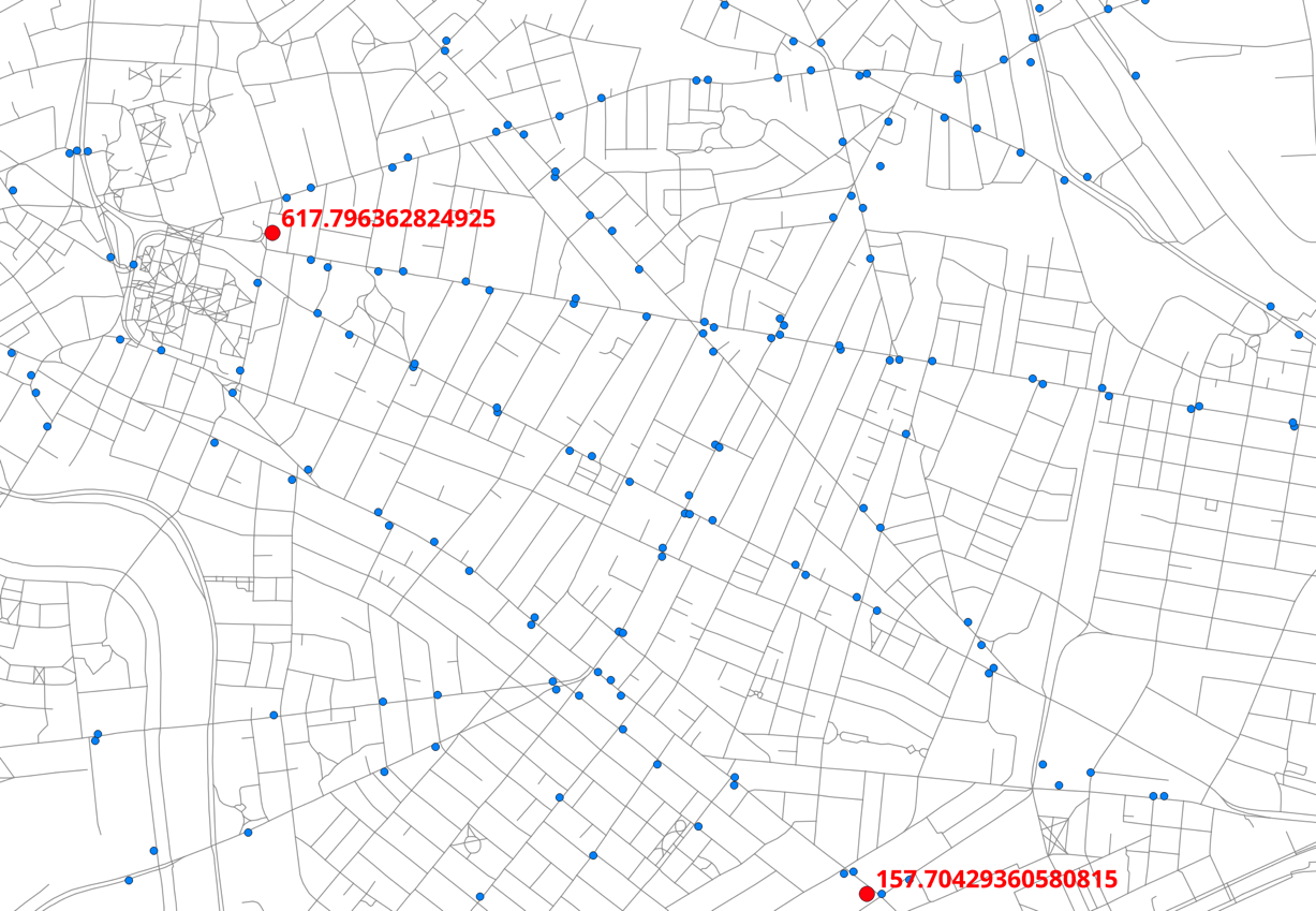
KNN is dominated by the single nearest stop: Harvard’s nearest stop has far higher weekly departures than MIT’s, so despite nearly identical Reach and Gravity totals, the KNN scores diverge sharply.
(f) Scale up — all 14,751 Cambridge building centroids
Same settings as (e), but computed for every building in Cambridge.
una.settings.origins_file = "Cambridge_building_centroids.geojson"
Metric |
n with access |
Mean |
Median |
p90 |
Max |
|---|---|---|---|---|---|
Reach |
13,135 |
3,197.96 |
2,490.00 |
5,986.00 |
20,027.00 |
Gravity (exp) |
13,135 |
2,451.64 |
1,864.02 |
4,572.85 |
16,457.07 |
Gravity (log) |
13,135 |
2,774.99 |
2,110.67 |
5,154.10 |
18,397.42 |
KNN access |
13,135 |
515.74 |
356.19 |
876.46 |
7,959.39 |

Gravity (exponential) per building centroid, visualized in QGIS.
About 89 % of buildings have at least one stop within a 400 m walk. The maxima belong to buildings near Harvard Square, Central Square, and Kendall Square where multiple bus and rail lines converge.
(g) Enable elevation, penalty = 4
Uphill walking accrues 4 extra cost-units per meter of rise. Swap in the 3D network (same 69,957 segments with SRTM 30 m z-values; elevation range −13 to 194 m):
una.settings.network_file = "20260703_PercLenNetwork_InnerCore_3D.geojson"
una.settings.elevation         = True
una.settings.elevation_penalty = 4
Metric |
n with access |
Mean |
Median |
p90 |
Max |
|---|---|---|---|---|---|
Reach |
12,897 |
2,967.93 |
2,241.00 |
5,548.20 |
19,934.00 |
Gravity (exp) |
12,897 |
2,277.92 |
1,726.00 |
4,313.34 |
16,027.12 |
Gravity (log) |
12,897 |
2,577.42 |
1,936.88 |
4,825.26 |
18,082.06 |
KNN access |
12,897 |
513.70 |
356.12 |
878.19 |
7,959.39 |
Served buildings drop ~1.8 % and mean Reach ~7 %, driven by uphill routes near Beacon Hill, Copp’s Hill, Bunker Hill, and the terrain rises in Somerville and Cambridge. MIT_SAP (flat river bank) is essentially unchanged; Harvard_GSD’s Reach falls ~15 % as some 400 m walks now climb toward the Radcliffe Yard rise.
(h) Enable turns, threshold = 45°, penalty = 35
Any deviation from straight-ahead by more than 45° at a node adds 35 cost-units. The turn-aware engine builds a line graph internally and is slower — expect a few minutes for all 14,751 origins. The tables below use the 2D network so they compare directly to step (f):
una.settings.network_file = "20260703_PercLenNetwork_InnerCore.geojson"
una.settings.elevation = False
una.settings.turns          = True
una.settings.turn_threshold = 45
una.settings.turn_penalty   = 35
Metric |
n with access |
Mean |
Median |
p90 |
Max |
|---|---|---|---|---|---|
Reach |
12,723 |
2,831.80 |
2,100.00 |
5,296.60 |
19,934.00 |
Gravity (exp) |
12,723 |
2,164.42 |
1,619.11 |
4,169.19 |
16,218.53 |
Gravity (log) |
12,723 |
2,455.62 |
1,831.23 |
4,713.00 |
18,281.50 |
KNN access |
12,723 |
513.13 |
353.85 |
872.96 |
7,951.62 |
Mean Reach falls ~11 % with turns enabled. Paths that look short on a map can become inaccessible once realistic pedestrian routing costs are applied — and turns + elevation stack additively if you also switch back to the 3D network.
(i) WalkScore-style composite with UNA_Batch.py
Steps (a)–(h) measured accessibility to one destination type at a
time. A WalkScore-style composite sums accessibility across many
destination categories — schools, transit, food, healthcare, parks —
into one number per origin. UNA_Batch.py does this from a single
pairings CSV: one row per category, each with its own
destinations_file, search_radius, knn_weights, decay
parameters and flags. The Boston table
(Boston/Boston_KNN_pairings.csv) lists 10 categories (arts, bus,
food & beverage, health, metro, parks, personal services, public
institutions, retail, schools), each with batch_composite_output
= TRUE and composited on knn_access.
The full UNA_Batch.py script — edit the three path constants and
the analysis type at the top, everything else stays as shipped:
from urban_network_analysis import UNA

# --------------------------------------------------------------
# EDIT THESE THREE VALUES
# --------------------------------------------------------------

DATA_FOLDER   = r"Boston"
PAIRINGS_FILE = r"Boston/Boston_KNN_pairings.csv"
OUTPUT_FOLDER = r"Boston/Results"

# Which analysis to run per row — must match the metric in your
# pairings CSV:
#   "accessibility"  — for reach / gravity_* / knn_access composites
#   "flow"           — for edge_flow or node_flow composites
ANALYSIS = "accessibility"

# --------------------------------------------------------------
# Run the batch (per-row files + optional composite file)
# --------------------------------------------------------------

una = UNA()
una.settings.data_folder   = DATA_FOLDER
una.settings.output_folder = OUTPUT_FOLDER

una.RunBatch(ANALYSIS, pairing_file=PAIRINGS_FILE)
All the per-category settings — destinations_file,
search_radius, knn_weights, decay parameters, calculate_*
flags, batch_composite_output, batch_composite_result_column —
come from the pairings CSV rows, not from the script. Run it with:
python UNA_Batch.py
The script builds the topology once per row, runs the accessibility
engine per category, and — because rows set
batch_composite_output = TRUE — assembles a single joint output
with one row per origin building whose final composite_sum column
adds the 10 category KNN scores into one WalkScore-style number.
Compositing is built into UNA.RunBatch — see
Project workflow — RunBatch() for the mechanics and
/user_guide/settings_reference:name for per-row naming.
Note
Composites are grouped by origins layer. All 10 rows here share the
same origins file, so the batch writes a single composite file.
A pairing table whose rows use several different origin layers
(e.g. “Homes to …” and “Jobs to …” rows) produces one composite
file per origin layer, each with its own composite_sum column —
see Project workflow — RunBatch().
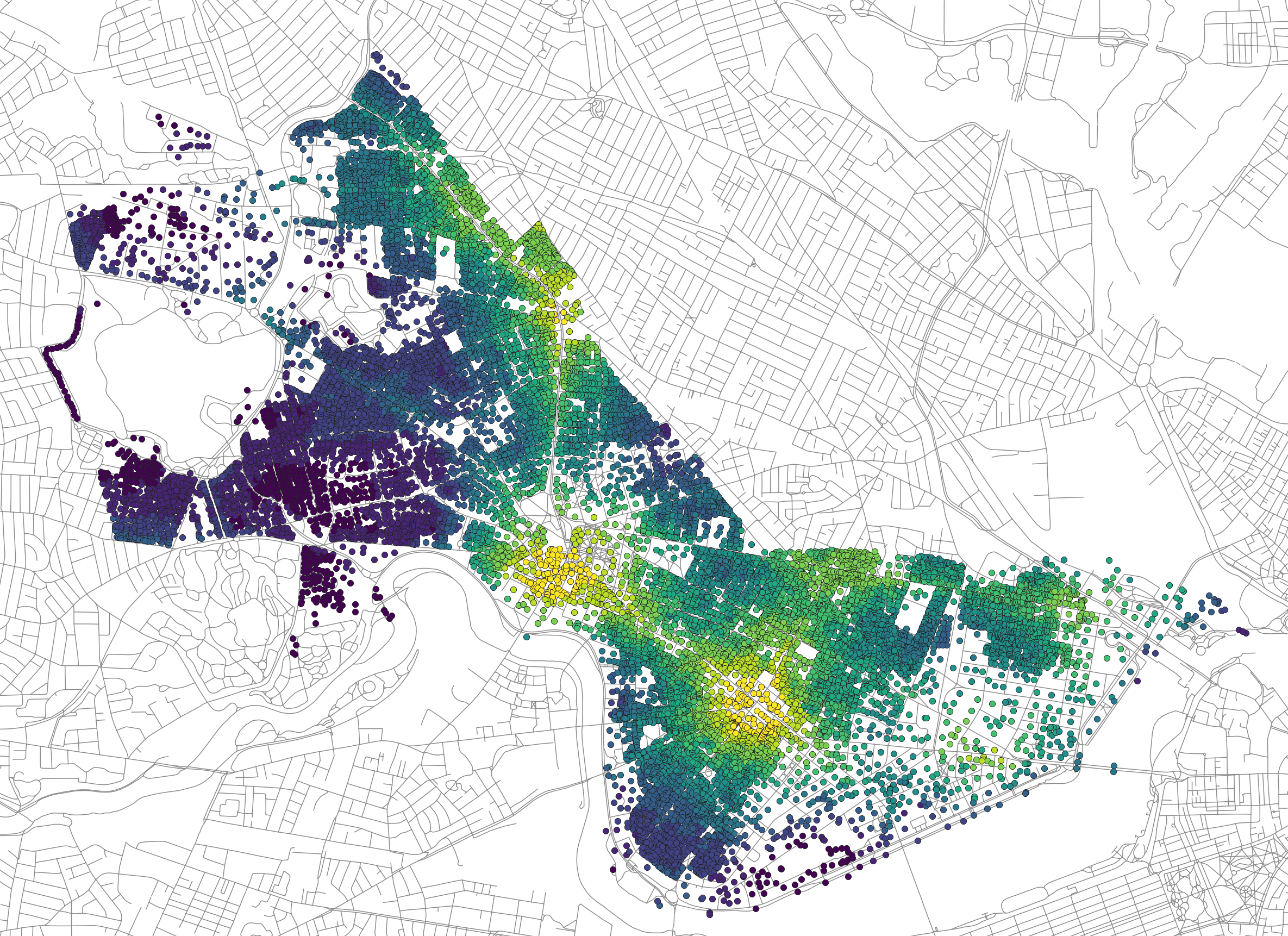
K-Nearest-Neighbor composite (WalkScore-style) for Cambridge building centroids. Highest scores near Harvard Square and Central Square.
Adapting the pairings table is the main editorial workflow: add a row
for a new category, tweak a radius or knn_weights vector, rerun —
no Python editing required. With turns=TRUE and elevation=TRUE
(3D network) the full 10-row run takes 30–60 minutes on a laptop; with
both FALSE, 5–10 minutes.
What we covered
Reach (a–b), Gravity under two decay shapes (c–d), KNN access (e),
city scale (f), elevation (g), turns (h), and a CSV-driven composite
(i). The same settings combine freely — try a different radius, a
sharper logistic midpoint, or knn_weights = (1.0, 1.0, 0.5) and
watch each change ripple through the result columns.
Next: Tutorial 3 — Foot-traffic flow analysis in Cambridge — from accessibility scores to per-edge pedestrian flows.